Build itPaste the brief into OpenCode and check that 23:00 → 01:00 gives +2 h.
OpenCode · development brief
Build a phase-comparison viewer: show before/after traces, let the reviewer click one peak per trace, compute the wrapped phase difference on a 24-h circle and show it on a dial. Export peaks and the difference.▎
Compare clock timing after a schedule changeSource & credit
Compare clock timing after a schedule change: Trace one comparison: choose a peak per trace → reference to the schedule → wrapped difference.
23:00 to 01:00 is two hours, not minus twenty-two. Owner-supplied illustrative interface; source figures credited below.
Cavallari et al. 2011, PLoS Biol — CC BY (reference actograms) (https://journals.plos.org/plosbiology/article/figure/image?size=large&id=10.1371/journal.pbio.1001142.g001)
Owner-supplied illustrative interface; source figures credited below.
Understand itTrace one nucleus: align frames → review spots → per-nucleus summary over time.
Input: frames + labels + schedule
↓Process: review, reject, summarise
↓Output: per-nucleus per-frame CSV
Choose toolsnapari for time-lapse layers, Python for summaries.
napari — layers over timePython — summariesNo LLM
Build itPaste the brief into OpenCode and verify a rejected spot disappears from the count.
OpenCode · development brief
Build a napari review for a nuclear time-lapse: show frames, nucleus labels and spot candidates, let the reviewer reject spots, and export per-nucleus spot counts per frame with the light condition attached.▎
Inspect photobodies as light conditions changeSource & credit
Inspect photobodies as light conditions change: Trace one nucleus: align frames → review spots → per-nucleus summary over time.
Spots per nucleus, frame by frame. Owner-supplied illustrative interface; source figures credited below.
Huang et al. 2016, eLife 5:e13292, Fig. 5B — CC BY 4.0 (https://iiif.elifesciences.org/lax:13292%2Felife-13292-fig5-v1.tif/full/full/0/default.jpg)
Owner-supplied illustrative interface; source figures credited below.
Understand itTrace one region: select → its trace → reviewed onset → compare with another region.
Input: regions + traces
↓Process: linked selection, onset review
↓Output: onset table
Choose toolsSVG for linked regions, Python for csv.
SVG — seedling regionsPython csv — tracesNo LLM
Build itPaste the brief into OpenCode and verify region selection filters correctly.
OpenCode · development brief
Build a linked seedling viewer: clickable regions from regions.json, the selected region's trace, a reviewer-set onset time per region and an onset comparison table with export.▎
Compare shoot-to-root signal timingSource & credit
Compare shoot-to-root signal timing: Trace one region: select → its trace → reviewed onset → compare with another region.
Pick a region, read its trace. Owner-supplied illustrative interface; source figures credited below.
Understand itTrace one tissue: review mask → check overlap → area and radial extent.
Input: section + masks + calibration
↓Process: overlap check, area, radial measurement
↓Output: table with areas that sum to the section
Choose toolsFiji for measurements, HTML/SVG for the viewer.
Fiji/ImageJ — masksHTML + SVG — viewerNo LLM
Build itPaste the brief into OpenCode and confirm synthetic tissue areas sum correctly.
OpenCode · development brief
Build a section viewer that overlays tissue masks, reports overlap, computes calibrated area and radial extent per tissue and exports a table whose tissue areas sum to the classified section.▎
Measure a stem's vascular tissue layersSource & credit
Measure a stem's vascular tissue layers: Trace one tissue: review mask → check overlap → area and radial extent.
Tissue areas that add up to the section. Owner-supplied illustrative interface; source figures credited below.
Lebovka et al. 2023, eLife 12:e66627, Fig. 2 — CC BY 4.0 (https://iiif.elifesciences.org/lax:66627%2Felife-66627-fig2-v2.tif/full/full/0/default.jpg)
Owner-supplied illustrative interface; source figures credited below.
Understand itTrace one step: allocate area → radius → ring.
Input: parameters
↓Process: per-step area allocation
↓Output: rings + table
Choose toolsJavaScript Math and SVG; no biological model.
JavaScript — mathsSVG — ringsNo LLM
Build itPaste the brief into OpenCode and run the two checks.
OpenCode · development brief
Build a radial-growth sandbox: parameters, per-step area allocation, derived radii and rings drawn per step with a table. Include tests for zero production and total-area conservation.▎
Explore a simple radial-growth modelSource & credit
Explore a simple radial-growth model: Trace one step: allocate area → radius → ring.
Understand itTrace one run: define reactions → simulate a supply → inspect trajectories.
Input: SBML + supply
↓Process: COPASI simulation
↓Output: species trajectories
Choose toolsCOPASI for the model, HTML/SVG for the viewer.
COPASI (Artistic-2.0)HTML + SVGNo LLM
Build itPaste the brief into OpenCode and check the declared balance.
OpenCode · development brief
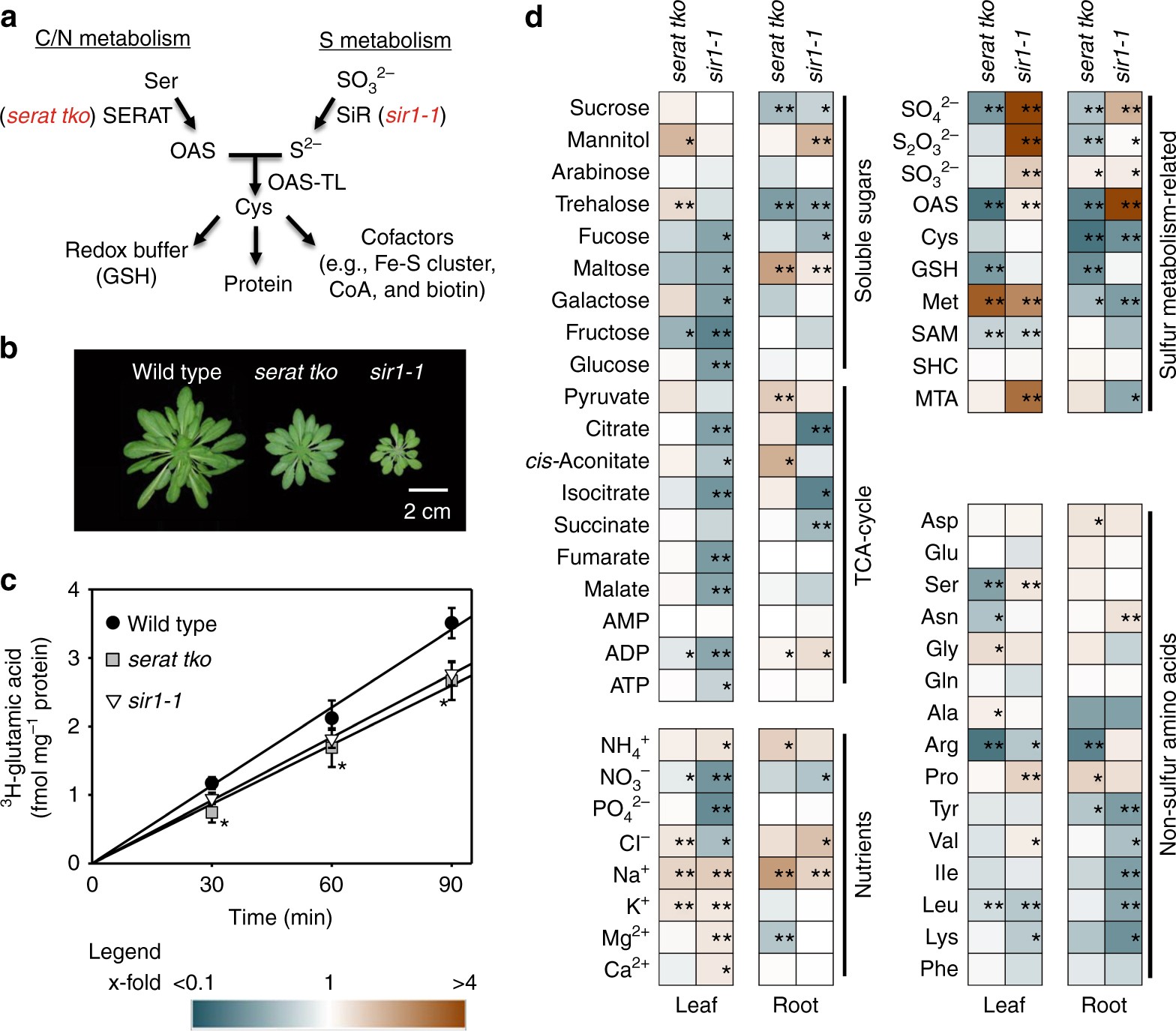
Build a reaction-model explorer: load COPASI CSV exports, show the reaction network and species trajectories for a chosen supply, and check the declared sulfur balance before allowing comparisons.▎
Explore a sulfur-metabolism modelSource & credit
Explore a sulfur-metabolism model: Trace one run: define reactions → simulate a supply → inspect trajectories.
Simulate one supply, watch every species. Owner-supplied illustrative interface; source figures credited below.
Dong et al. 2017, Nat Commun 8:1174 — CC BY 4.0 (https://media.springernature.com/full/springer-static/image/art%3A10.1038%2Fs41467-017-01224-w/MediaObjects/41467_2017_1224_Fig1_HTML.jpg)
Owner-supplied illustrative interface; source figures credited below.
↓Output: highlighted subgraph + a path list that cites the synapse rows
Choose toolsJavaScript adjacency lists and SVG; the published graph image as the hero, the tables as the truth.
JavaScript Map — adjacency listsSVG — force layout or fixed positions from the paperNo LLM
Build itPaste the brief into OpenCode and verify directionality with a known one-way connection.
OpenCode · development brief
Build a connectome explorer from neurons.csv and synapses.csv. Let the user select a neuron, show its pre- and postsynaptic partners with synapse counts, trace a directed path between two neurons, colour nodes by module,▎
Trace a larval neural circuitSource & credit
Trace a larval neural circuit: Trace one neuron: validate its ID → list partners → walk a directed path, each hop backed by a synapse row.
Understand itTrace one record: validate coordinates → draw a halo sized by its uncertainty → link the point to its record.
Input: GBIF records with coordinate uncertainty
↓Process: validate, filter by licence/year, project, draw halo + point
↓Output: linked map and record panel; excluded records are not drawn
Choose toolsPython for fetching and validation, browser SVG for the map; GBIF API and Natural Earth as data sources.
GBIF occurrence API — records (data licence per dataset: CC0 / CC BY / CC BY-NC)Natural Earth — outlines, public domainPython csv — validation and licence filter
Build itPaste the brief into OpenCode, fetch the records and verify that no excluded record appears on the map.
OpenCode · development brief
Build an occurrence map for one species from a GBIF CSV. Draw each record as a point with a halo scaled to its coordinate uncertainty, mark records without uncertainty distinctly, filter by year and licence, and open the▎
Map plant records with their uncertaintySource & credit
Map plant records with their uncertainty: Trace one record: validate coordinates → draw a halo sized by its uncertainty → link the point to its record.
Map plant records with their uncertainty. Owner-supplied illustrative interface; source figures credited below.
GBIF occurrence API (records CC0 / CC BY 4.0, accessed 2026-09-10) (https://api.gbif.org/v1/occurrence/search?taxonKey=3052436&hasCoordinate=true&license=CC0_1_0&license=CC_BY_4_0)
Natural Earth 1:50m countries — public domain (https://github.com/nvkelso/natural-earth-vector)
Krämer 2015, eLife 4:e06100, Fig. 3 — A. thaliana range map, CC BY 4.0 (https://iiif.elifesciences.org/lax:06100%2Felife-06100-fig3-v1.tif/full/full/0/default.jpg)
Owner-supplied illustrative interface; source figures credited below.
Understand itTrace one trait: select comparable units → group by documented ploidy → inspect variation.
Input: three tables
↓Process: group, keep unknown separate
↓Output: matrix + source rows
Choose toolsPython for grouping, HTML/SVG for the matrix.
Python csvHTML + SVGNo LLM
Build itPaste the brief into OpenCode and confirm unknown ploidy stays separate.
OpenCode · development brief
Build a ploidy × trait explorer: join accessions, ploidy evidence and traits, group by documented ploidy with an explicit unknown group, show a matrix with n per cell and the source rows on click, and export.▎
Compare plant traits across ploidy groupsSource & credit
Compare plant traits across ploidy groups: Trace one trait: select comparable units → group by documented ploidy → inspect variation.
Unknown ploidy is its own group. Owner-supplied illustrative interface; source figures credited below.
Thomas Kraehahn, Wikimedia Commons — CC BY 4.0 (https://commons.wikimedia.org/wiki/File:Sand-Schaumkresse_im_NSG_Erpetal.jpg)
Owner-supplied illustrative interface; source figures credited below.
Choose toolsPython for joins, HTML/SVG for the matrix.
Python csvHTML + SVGNo LLM
Build itPaste the brief into OpenCode and verify the binding-only row.
OpenCode · development brief
Build a target-gene evidence browser: join assays, contrasts and evidence, show a gene × layer matrix by tissue, keep binding and expression layers separate, and export a shortlist.▎
Explore Hox targets by tissue and stageSource & credit
Explore Hox targets by tissue and stage: Trace one gene: select contrasts → inspect evidence layers → shortlist.
Binding is not expression. Owner-supplied illustrative interface; source figures credited below.
Domsch et al. 2019, eLife 8:e42675, Fig. 3 — CC BY 4.0 (https://iiif.elifesciences.org/lax/42675%2Felife-42675-fig3-v3.tif/full/full/0/default.jpg)
Owner-supplied illustrative interface; source figures credited below.
Understand itTrace one marker: join → colour → inspect a subset.
Input: geometry + markers
↓Process: join, colour, select
↓Output: map + linked details
Choose toolsSVG for the map; napari optional.
SVG + JavaScriptnapari (optional)No LLM
Build itPaste the brief into OpenCode and verify missing values are not coloured as zero.
OpenCode · development brief
Build a meristem cell map: draw cells from geometry, colour by a chosen marker with a sequential scale, show missing values as dashed outlines, allow region selection with linked details and export.▎
Map markers across a shoot meristemSource & credit
Map markers across a shoot meristem: Trace one marker: join → colour → inspect a subset.
Missing value ≠ zero, on every cell. Owner-supplied illustrative interface; source figures credited below.
Schlegel et al. 2021, eLife 10:e70934, Fig. 2 — CC BY 4.0 (https://iiif.elifesciences.org/lax:70934%2Felife-70934-fig2-v2.tif/full/full/0/default.jpg)
Owner-supplied illustrative interface; source figures credited below.